Technical Deep-Dive
The bank-marketing classifier had to clear three hurdles at once: an 88.6 / 11.4 class split, errors that don’t cost the same (a wasted call is cheap, a missed deposit is expensive), and a target metric that lives outside the standard sklearn report — campaign dollars, not accuracy. This page walks through the data preparation, the three models we trained, and the cost-sensitive evaluation we used to compare them.
Every code excerpt below is a verbatim cut from the actual training script. Click “View on GitHub →” above any block to open the full file in the repo.
Dataset
- Source: UCI Bank Marketing dataset
- Size: 37,069 client records · 20 features
- Target:
y ∈ {yes, no}— did the client subscribe to a term deposit? - Class balance: 88.6% no / 11.4% yes
- Features: demographics (age, job, marital, education), prior contact history (
campaign,pdays,previous,poutcome), and macroeconomic indicators (emp.var.rate,cons.price.idx,cons.conf.idx,euribor3m,nr.employed)
Feature engineering and leakage prevention
Two preprocessing steps apply across all three models.
pdays = 999 recoded as a binary flag. The raw column encodes “days since last contact,” but uses the sentinel 999 for clients never contacted before. Treating that as a number breaks any distance-based model (KNN especially). We replace it with a clean binary never_contacted feature.
month dropped to prevent temporal leakage. Month-of-year is heavily correlated with macroeconomic indicators and with the campaign itself — it leaks information about which campaign a record came from rather than about the client. Dropping it forces the model to learn client-level signal.
campaignData['never_contacted'] = np.where(
    campaignData['pdays'] == 999,
    1,
    0
)

campaignData = campaignData.drop('pdays', axis=1)

X = campaignData.drop(['y', 'month'], axis=1)

X_encoded = pd.get_dummies(X, drop_first=True)
Categoricals are one-hot encoded with drop_first=True (Models 1 & 2) or with OneHotEncoder(drop='first') inside a pipeline (Model 3). Dropping the reference level avoids the dummy-variable trap without losing information.
Handling class imbalance
We tried three different strategies and let the cost-sensitive evaluation tell us which worked best.
SMOTE oversampling. Synthetic Minority Oversampling Technique fabricates new positive-class samples by linearly interpolating between existing positives and their k-nearest minority neighbors in feature space. It’s applied after the train/test split (otherwise the test set leaks into training). Used in Models 1 & 2.
Automatic class weighting. class_weight='balanced' reweights the loss inversely to class frequency — a misclassified positive contributes ~7.8× as much to the loss as a misclassified negative on this dataset. This shifts the decision boundary toward the minority class without inventing synthetic data. Used in Models 2 & 3.
Probability threshold tuning. Rather than accepting sklearn’s default 0.5 cutoff, Model 3 predicts probabilities and applies a tuned threshold of 0.61. Raising the threshold trades recall for precision — fewer positive predictions, but each one is more likely to be a real subscription. This is the most direct lever for a cost-asymmetric problem.
Cost-sensitive evaluation
Accuracy is the wrong metric. A classifier that always says “no” hits ~89% accuracy and generates zero revenue. We defined a custom campaign value function rooted in operational economics:
| Parameter | Value | Source |
|---|---|---|
| Employee wage | ~$11 / hr | Bank operations |
| Average call duration | ~30 min | Historical campaign data |
| Average savings deposited | ~$4,960 | Subscriber profile |
| Term-deposit allocation | 75% | Bank policy |
| Net interest margin | 1.2% | Bank financials |
| Value per true positive | +$44.64 | $4,960 × 75% × 1.2% |
| Cost per wasted call | –$5.50 | 30 min × $11/hr |
Campaign value is then (TP × $44.64) − (calls × $5.50). A model that makes fewer, more precise calls can outperform one with higher recall. This is the metric we tune for.
Three model variants
Model 1 — Random Forest with SMOTE
The baseline ensemble approach: oversample the minority class to balance the training set, then train a Random Forest with manual class weights and conservative tree depth to prevent overfitting on the synthetic samples.
smote = SMOTE(random_state=42)

X_train_resampled, y_train_resampled = smote.fit_resample(X_train, y_train)

refined_model = RandomForestClassifier(
    max_depth=5,
    min_samples_leaf=10,
    min_samples_split=20,
    class_weight={0: 1, 1: 1.5},
    random_state=42
)

refined_model.fit(X_train_resampled, y_train_resampled)
Result: Broadest call list — 129 calls on the mini-holdout, catching the most true positives (31) but at the lowest precision (24.0%), which dilutes per-call value.
Model 2 — Random Forest with balanced class weights
Same pipeline as Model 1 but with one structural change: instead of manual {0: 1, 1: 1.5} weights, use sklearn’s 'balanced' mode, which sets weights as n_samples / (n_classes × n_class_i). On this dataset that resolves to roughly {0: 0.56, 1: 4.4} — a much stronger penalty on misclassified positives.
model = RandomForestClassifier(
    max_depth=5,
    min_samples_leaf=10,
    min_samples_split=20,
    class_weight='balanced'
)

model.fit(X_train_resampled, y_train_resampled)
Result: Tighter call list — 82 calls, precision 34.1%, and the best projected total value at scale ($7,775 on a 4,119-contact campaign). Higher per-call efficiency than Model 1 because the heavier class penalty drives the trees toward purer positive-class splits.
Model 3 — Stacking classifier (Random Forest + KNN)
The most ambitious variant. Two base learners with complementary inductive biases — Random Forest (axis-aligned, global splits) and K-Nearest Neighbors (local, distance-based decisions) — feed their predictions into a Logistic Regression meta-learner. Cross-validated stacking ensures the meta-learner isn’t trained on the base learners’ in-sample predictions.
preprocessor = ColumnTransformer(
    transformers=[
        ('num', StandardScaler(), numerical_features),
        ('cat', OneHotEncoder(drop='first'), categorical_features)
    ]
)

rf = Pipeline([
    ('preprocessor', preprocessor),
    ('rf', RandomForestClassifier(n_estimators=10, max_depth=5,
                                  n_jobs=-1, class_weight='balanced'))
])

knn = Pipeline([
    ('preprocessor', preprocessor),
    ('knn', KNeighborsClassifier(n_neighbors=3, n_jobs=-1))
])

base = [
    ('rf', rf),
    ('knn', knn)
]

meta = LogisticRegression(max_iter=20, class_weight={0: 1, 1: 4})

stacking_clf = StackingClassifier(
    estimators=base,
    final_estimator=meta,
    cv=3,
    n_jobs=-1
)
Three things to note about this construction.
Each base learner is wrapped in its own Pipeline so the preprocessor is fit within each cross-validation fold during stacking — no leakage. The StandardScaler matters specifically for KNN (Euclidean distances are scale-sensitive); the RF doesn’t care, but bundling them together keeps the pipeline uniform.
The KNN classifier is set to n_neighbors=3 — small enough to capture local pockets of subscribers (e.g., retirees in a specific economic regime) without smoothing them away. Combined with class_weight='balanced' on the RF, the two base learners produce probability estimates from very different views of the data.
The meta-learner is a LogisticRegression with class_weight={0: 1, 1: 4} — another layer of class weighting, this time applied to the base learners’ output probabilities. The combination of base-level weighting and meta-level weighting is what lets the model push precision past 47% while still catching 25 of 47 positives.
After training, predictions go through a tuned threshold of 0.61 rather than sklearn’s default 0.5:
y_pred_proba = stacking_clf.predict_proba(X_test)[:, 1]

threshold = 0.61
y_pred = (y_pred_proba >= threshold).astype(int)
Result: Most selective call list — 53 calls, 47.2% precision, and the best per-call value at $15.56. The stacking architecture lets the KNN’s local neighborhood patterns complement the Random Forest’s global splits, and the threshold tuning concentrates the calls on only the most confident positives.
Side-by-side results
Recent 410-contact test campaign
| Model | Calls | TP | Precision | Campaign Value |
|---|---|---|---|---|
| No model (call everyone) | 410 | 47 | 11.5% | –$156.92 |
| Model 1 — RF + SMOTE | 129 | 31 | 24.0% | $674.34 |
| Model 2 — RF balanced | 82 | 28 | 34.1% | $798.92 |
| Model 3 — Stacking | 53 | 25 | 47.2% | $824.50 |
Value per call
| Model | Value / Call | Lift vs. baseline |
|---|---|---|
| Model 3 — Stacking | $15.56 | +$15.94 |
| Model 2 — RF balanced | $9.74 | +$10.13 |
| Model 1 — RF + SMOTE | $5.23 | +$5.61 |
| No model | –$0.38 | — |
Projected full campaign (4,119 contacts)
| Model | Projected calls | Projected value |
|---|---|---|
| Model 2 — RF balanced | 798 | $7,774.86 |
| Model 3 — Stacking | 484 | $7,529.40 |
| Model 1 — RF + SMOTE | 1,268 | $6,628.40 |
| No model | 4,119 | –$1,576.47 |
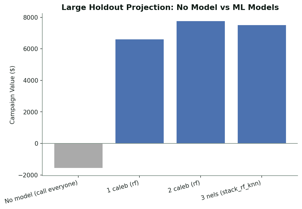
Campaign value across the holdout set, with and without model filtering.
How the call list is reshaped
The model doesn’t just pick fewer people — it picks different people. It systematically concentrates outreach on three high-conversion segments and prunes three low-conversion ones.
| Segment | Without ML | With Model 3 | Shift |
|---|---|---|---|
Previously converted (poutcome: success) |
2.9% | 20.8% | +17.8 pp |
Retirees (job: retired) |
4.9% | 22.6% | +17.8 pp |
Students (job: student) |
2.9% | 9.4% | +6.5 pp |
Reached by landline (contact: telephone) |
37.1% | 9.4% | −27.6 pp |
Blue-collar workers (job: blue-collar) |
20.7% | 1.9% | −18.8 pp |
Basic education, 9 yr (education: basic.9y) |
15.9% | 1.9% | −14.0 pp |
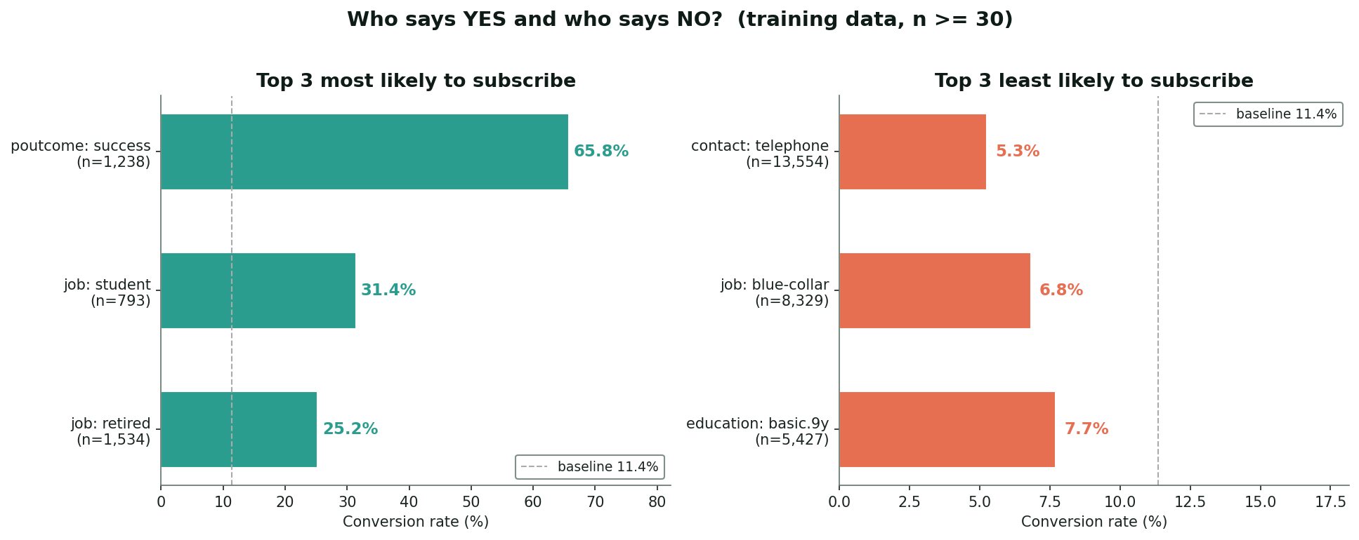
Conversion rates by segment and the model’s reshape of the call list.
Trade-offs and choosing between models
Both Model 2 and Model 3 are “right” answers depending on the operational constraint.
Use Model 3 when call capacity is the bottleneck. Best per-call efficiency ($15.56) and highest precision (47.2%). Optimal when you have a fixed number of agent-hours and need every minute to count.
Use Model 2 when you can staff up. Highest projected total value ($7,775 on 4,119 contacts) because it casts a wider net — it accepts a precision hit to catch more positives in absolute terms.
Both models cleanly flip the campaign from money-losing to profitable. Model 1 (SMOTE + RF) is dominated by Model 2 across every metric and is included primarily as a methodological baseline showing what oversampling adds (or doesn’t) when stronger class-weighting is available.
Code, data, and reproduction
- Training scripts:
module_2-bank/models/ - Training data:
module_2-bank/training_data/bank.csv - Holdout predictions:
module_2-bank/predictions/ - Visualisation source:
module_2-bank/visualisation/ - Verification notebook:
module_2-bank/verification/
To reproduce locally: clone the repo, pip install -r requirements.txt (scikit-learn, imbalanced-learn, polars, pandas), then run any of the three scripts from inside module_2-bank/models/. Each script writes its holdout predictions to module_2-bank/predictions/ and prints a classification report and top-feature importances to stdout.